R code (knitr)

Overleaf provides an integration with knitr, which allows you to add R code to your LaTeX document to generate a dynamic output.

Documents that contain R code must be saved with the extension .Rtex or .Rnw, otherwise the code won’t work. Let’s see an example:

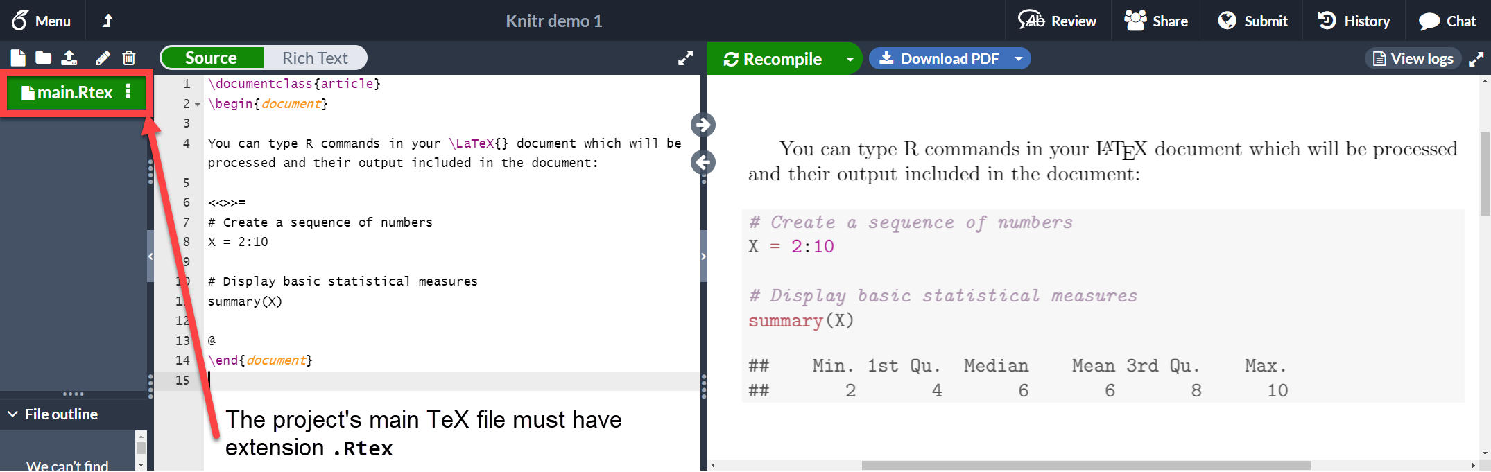
\documentclass{article}
\begin{document}

You can type R commands in your \LaTeX{} document which will be processed and their output included in the document:

<<>>=
# Create a sequence of numbers
X = 2:10

# Display basic statistical measures
summary(X)

@
\end{document}

Open this knitr example on Overleaf

As you can see, the text in between the characters <<>>= and @ is R code. This code and its output is printed in a listing-like format. This chunk of code can take some extra parameters to customize the dynamic output, as described in the next section.

Chunks of code

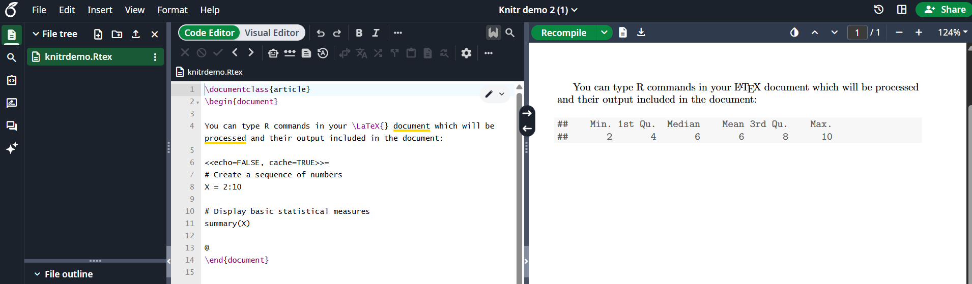
A code block like the one presented in the previous section is usually called a chunk. You can set some extra options in knitr chunks. See the example below:

\documentclass{article}
\begin{document}

You can type R commands in your \LaTeX{} document which will be processed and their output included in the document:

<<echo=FALSE, cache=TRUE>>=
# Create a sequence of numbers
X = 2:10

# Display basic statistical measures
summary(X)

@
\end{document}

Open this knitr example on Overleaf

There are two additional options passed inside << and >>.

• echo=FALSEThis hides the code and only prints the output generated by R.

• cache=TRUEIf cache is set to true, the chunk is not run, only the objects generated by it. This saves time if the data in that chunk haven’t changed.

  Note that the cache=TRUE option is not currently supported in Overleaf, but it should work locally.

See the reference guide for more options.

Inline commands

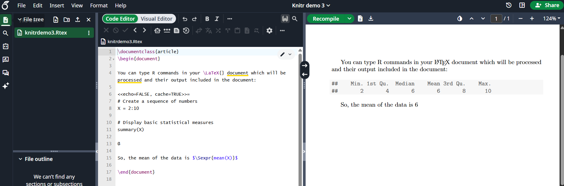
It is possible to access objects generated in a chunk and print them in-line.

\documentclass{article}
\begin{document}

You can type R commands in your \LaTeX{} document which will be processed and their output included in the document:

<<echo=FALSE, cache=TRUE>>=
# Create a sequence of numbers
X = 2:10

# Display basic statistical measures
summary(X)

@

So, the mean of the data is $\Sexpr{mean(X)}$
\end{document}

Open this knitr example on Overleaf

The command \Sexpr{mean(X)} prints the output returned by the R code mean(X). Inside the braces, any R command can be passed.

Plots

Plots can also be added to a knitr document, as in this example:

\documentclass{article}
\begin{document}

<<plot1, fig.pos="t", fig.height=4, fig.width=4, fig.cap="First plot">>=

xdata = read.csv(file="data.txt", head=TRUE,sep=" ")

hist(xdata$data, main="Overleaf histogram", xlab="Data")

@

The figure \ref{fig:plot1} is simple histogram.

\end{document}

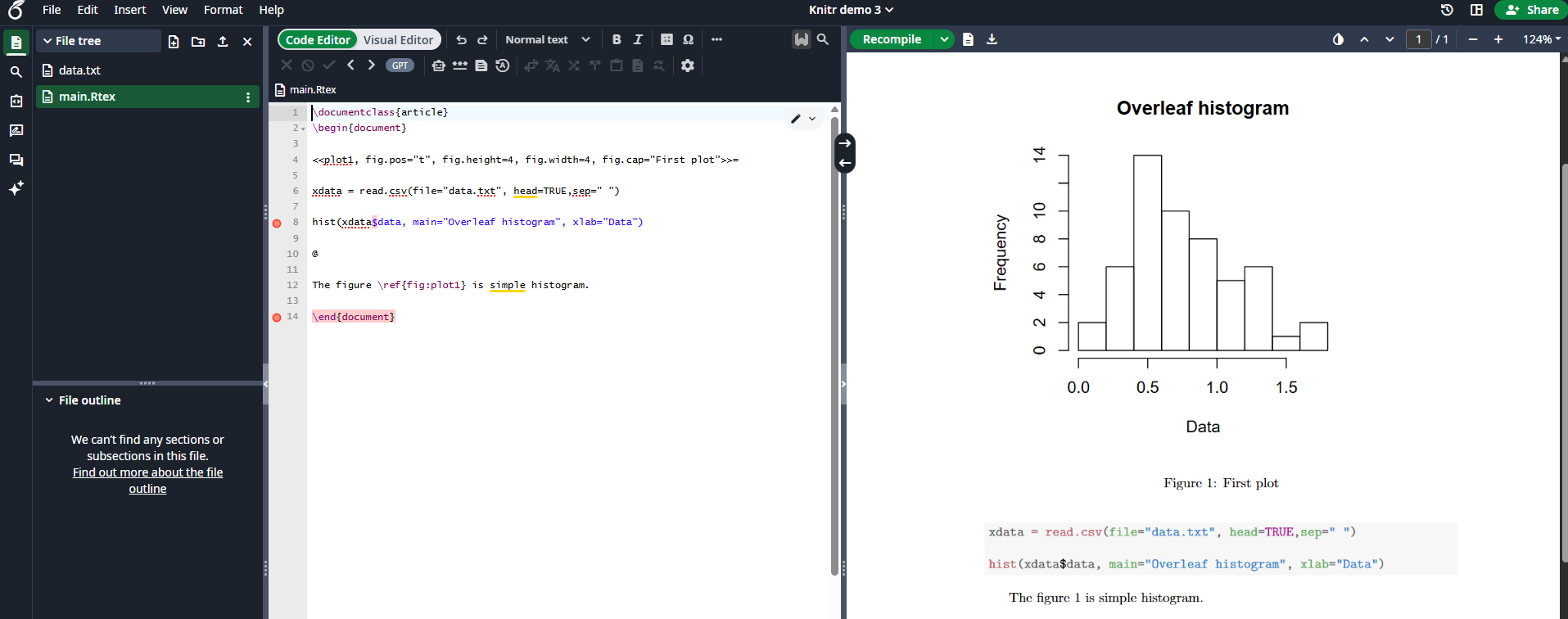
Open this knitr example on Overleaf

This histogram uses data stored in “data.txt”, saved in the current working directory. A few figure-related options are passed to the chunk.

plot1This is the label used to reference the plot. The prefix “fig:” is mandatory. You can see in the example that the figure is referenced with \ref{fig:plot1}.fig.pos="t" positioning parameter. This is the same used in the figure environment.fig.height=4, fig.width=4Figure width and height.fig.cap="First plot"Caption for the figure.

External R scripts

You can import parts of an external R script into a knitr document. This is very helpful since it is fairly common to write and debug the script in an external program prior to including it in your document.

Suppose we have the following R code in a file called mycode.R which we include in our LaTeX document:

## ---- myrcode1
# Create a sequence of numbers
 X = 2:10

## ---- myrcode2
# Display basic statistical measures
summary(X)

Notice the lines:

## ---- myrcode1

and

## ---- myrcode2

These mark the beginning of a chunk of code and are mandatory if you want to use this script in our document, as shown in the following code fragment:

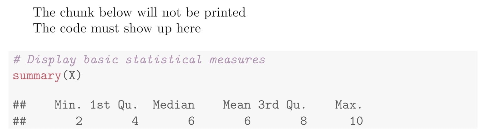
The chunk below will not be printed

<<echo=FALSE, cache=FALSE>>=
read_chunk("mycode.R")
@

The code must show up here

<<myrcode2>>=

@

The first chunk is not printed and is only used to import the script with the command read_chunk("mycode.R") . That’s why the option echo=FALSE is set. Also, scripts must not be cached. Once the script is imported, you can print a chunk using the label you set after ## ----. In this case it’s myrcode2.

We have put all the article code fragments into a project that you can Open on Overleaf .

Reference guide

Some chunk options:

• results. Changes the behavior of the results generated by the R code. Possible values are:
  • markup Use LaTeX to format the output.
  • asis Print raw results from R.
  • hold Hold the output results and push them to the end of the chunk.
  • hide Hide results.
• echo. Whether to include the R source code. Other parameters include:
  • echo=2:3 prints only the second and third lines;
  • echo=-2:-3 excludes the second and third lines only.
• cache. Whether to cache the code chunk. Possible values are: TRUE and FALSE
• highlight. Whether to highlight the source code. Possible values are: TRUE and FALSE
• background. Background color of the chunk. rgb and HTML formats can be used. The default value is “#F7F7F7”.